Image segmentation is one of the hotspots in image processing and computer vision and is also very important in image recognition. One of the most known and powerful approaches in image segmentation is the convolutional neural network (CNN). There are different approaches for image segmentation.
In this post, the thresholding method, clustering based methods and edge based methods are presented. In addition there are the very popular and powerful CNN and Laplacian based methods. In image segmentation we try to divide an image into different regions which are of interest. Pixel values which are close by and are similar are assigned to a group. If two neighbour pixels have divergent values, they are assigned to different categories. We first load the functions and packages needed. We mainly use skimage, which is used in python for image processing. In addition numpy and sklearn are loaded as well.
import numpy as np
from skimage import io
from skimage import filters
from skimage import color
from scipy import ndimage
from matplotlib.colors import LogNorm
import matplotlib.pyplot as plt
from sklearn.cluster import KMeans
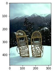
snow_pic=io.imread("2018.jpg")
plt.figure()
plt.imshow(snow_pic)
<matplotlib.image.AxesImage at 0x7f7b5b6c3110>
snow_pic.shape
(481, 321, 3)
The image used for image segmentation is from the Berkeley Segmentation Dataset. The image is of size 481*321 and has three RGB channels.
snow_gray=color.rgb2gray(snow_pic)
To ease the computation, the image is converted to a greyscale image and the greyscale image is used for further analysis.
plt.figure()
plt.imshow(snow_gray)
<matplotlib.image.AxesImage at 0x7f7b5b675c90>
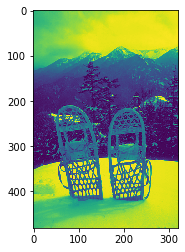
Imshow displays the values in a heatmap style instead of a greyscale. By using the option cmap=“gray”, the image is shown as a greyscale image. We will use a image thresholding called Otsu’ method.
val=filters.threshold_otsu(snow_gray)
mask=snow_gray<val
plt.figure()
plt.imshow(mask)
<matplotlib.image.AxesImage at 0x7f7b5b5da990>
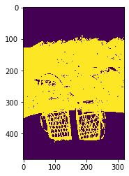
Otsu’s Method is used for calculating an image-thresholding. Otsus’s method assumes that an image consists of two classes of pixels, foreground and background pixel. It calculates the optimal value for minimizing the intra-class variance for both groups. If we just apply Otsu’s filter, the image is divided into two segments. The filter is very blurry and it can not really distinguish between the snow shoes and the trees in the background. For this picture this method is clearly inadequate and we need something more sophisticated.
KMeans for image segmentation
Another widely used algorithm for image segmentation is kmeans. Kmeans is a clustering algorithm which assigns an observation to the nearest cluster center. After the assignment it calculates the new cluster center for the new observations. For the new cluster center the observation are again assigned to the nearest cluster center. This process is done iteratively until the solution does not change. The number of clusters need to be defined before, which is a disadvantage of KMeans. We will later try to find the optimal number of clusters. But in this example we set the number of clusters to 10.
ll=KMeans(10).fit(snow_gray.reshape(-1,1))
ll=ll.predict(snow_gray.reshape(-1,1))
fig, (ax1,ax2)=plt.subplots(ncols=2,nrows=1,figsize=(10,8))
ax1.imshow(snow_pic)
ax1.set_title("Original")
ax2.imshow(ll.reshape(481,321))
ax2.set_title("Kmeans Solutions for 10 Cluster")
Text(0.5, 1.0, 'Kmeans Solutions for 10 Cluster')
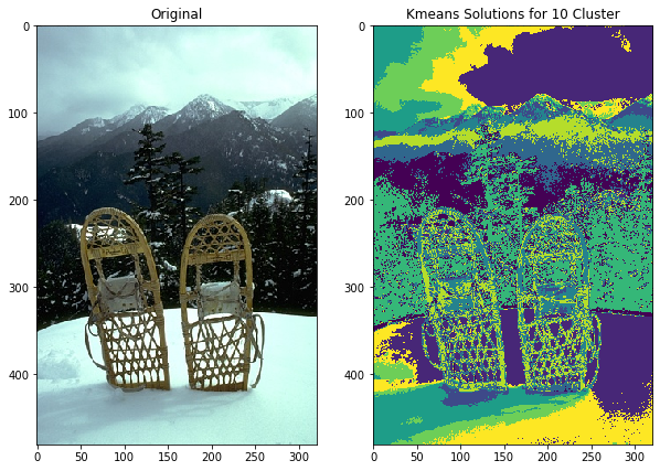
We use the KMeans function to calculate the solution for 10 clusters as an example. We use the predict method for obtaining the cluster solution and plot the correpsonding solution. The right image shows the cluster solution and we can see that the image is not well clustered. The snow shoes are somewhat visible but the forest in the background is hardly visible. As a way of deciding how many clusters we need we use the scree plot. In this example we calculate the KMeans solution for one to 30 clusters and extract the score.
value=[]
n=30
for i in range(1,n):
    kmeans=KMeans(i).fit(snow_gray.reshape(-1,1))
    value.append(kmeans.score(snow_gray.reshape(-1,1)))
The idea of the scree plot is to calculate for different number of clusters the total within squares of sum. This is a measure of total dispersion and indicates how similiar these clusters are. The within sum of squares decreases with the number of clusters added but quite often we see a sharp bend in this plot, which indicates the total number of optimal clusters.
plt.figure()
plt.plot(range(1,30),value)
[<matplotlib.lines.Line2D at 0x7f7b5b4fcc90>]
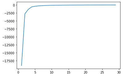
In this plot we see a sharp bend for five clusters. The optimal number of clusters is right before the “elbow” bend. In this case the optimal solutions seems to be four clusters.
ll=KMeans(4).fit(snow_gray.reshape(-1,1))
ll=ll.predict(snow_gray.reshape(-1,1))
fig, (ax1,ax2)=plt.subplots(ncols=2,nrows=1,figsize=(10,8))
ax1.imshow(snow_pic)
ax1.set_title("Original")
ax2.imshow(ll.reshape(481,321))
ax2.set_title("Kmeans Solutions for 4 Cluster")
Text(0.5, 1.0, 'Kmeans Solutions for 4 Cluster')
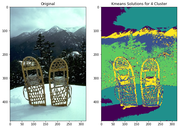
The Kmeans solution for four cluster seems to provide a good image segmentation. The snow shoes are visible as well as the forest and the mountains in the background. The shadow in front of the shoes are also visble as a distinct group.
Edge detection using the Sobel Filter
Edge detection is a useful method for detecting different regions in an image. The idea is to use the gradient of the greyscales. For discontinous values we can assume this is due to two different regions in the image. In the image above the greyscale values between the shoes and the snow would show a drastic change of the greyscale values. On the other hand the greyscale values of the snow in the bottom of the image are similiar or exactly the same. We would therefore conclude that the pixels belong to the same region in the image. To detect these edges, filters and convolutions are used. The idea of convolution is to use a matrix of certain size for example 3*3 to discover horizontal,vertical or diagonal edges.
\[\begin{bmatrix}-1 & 0 & 1 \\ -2 & 0 & 2 \\ -1 & 0 & 1 \\ \end{bmatrix}\]
The matrix above is an example of a 3*3 convolution matrix. This convolution filter detects edges in x direction. The filter is placed on each pixel of the image, than the pixels around the center are calculated using the matrix. This calculated value is the new value and the filter is placed on the next pixel. This is done for the whole image.
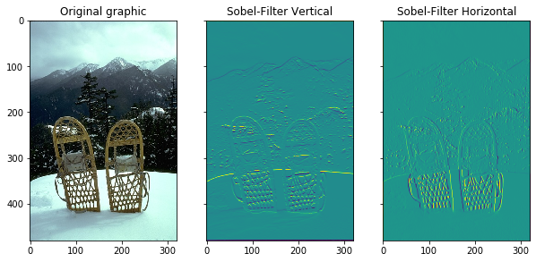
The Sobel Edge detector is using gradients for extracting corners. It calculates the derivatives for the x and y axis seperately. The mode parameter is needed in case the filter crosses a border. With mode set to constant, all values outside the border of the image have a constant value which can be set by the parameter cval. The default value is set to 0. With axis the direction of the filter can be set. In this case edges in horizontal and vertical directions are detected.
dx=ndimage.sobel(snow_gray,axis=0,mode="constant")
dy=ndimage.sobel(snow_gray,axis=1,mode="constant")
fig, (ax1,ax2,ax3)=plt.subplots(nrows=1, ncols=3, figsize=(10, 6),
                                    sharex=True, sharey=True)
ax1.imshow(snow_pic)
ax1.set_title("Original graphic")
ax2.imshow(dx)
ax2.set_title("Sobel-Filter Vertical")
ax3.imshow(dy)
ax3.set_title("Sobel-Filter Horizontal")
Text(0.5, 1.0, 'Sobel-Filter Horizontal')
The original image and the Sobel filter for the x and y direction are plotted. We can also calculate the strength or magnitude and the orientation of the filter. The magnitude is defined in the following way:
\[\sqrt{G_x^2+G_y^2}\]
where \(G_x^2\) is the square of the gradient in x-direction. In this case these are discrete values. The magnitude can be approximated by using the absolute values for the x and y direction and than taking the sum. The orientation of an image is defined this way:
\[tan^{-1}(\frac{G_X}{G_Y})\]
orientation=np.arctan2(dx,dy)
mag=np.sqrt(np.power(dx,2)+np.power(dy,2))
The first line calculates the orientation and the second line calculates the magnitude of the image, by using the formulas mentioned before.
fig, ([ax1, ax4], [ax5,ax6]) = plt.subplots(nrows=2, ncols=2, figsize=(12, 8),
                                    sharex=True, sharey=True)
ax1.imshow(snow_pic)
ax1.set_title("Original graphic")
#ax2.imshow(dx)
#ax2.set_title("Sobel-Filter Vertical")
#ax3.imshow(dy)
#ax3.set_title("Sobel-Filter Horizontal")
ax4.imshow(dx.__abs__()+dy.__abs__())
ax4.set_title("Sobel-Filter Approximate Sum")
ax5.imshow(dx.__abs__()+dy.__abs__())
ax5.set_title("Sobel-Filter Sum")
ax6.imshow(orientation,cmap="gray")
ax6.set_title("Sobel-Filter Orientation")
Text(0.5, 1.0, 'Sobel-Filter Orientation')
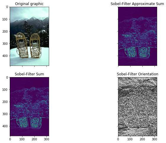
In this graphic the original image, the approximate sum, the exact sum and the orientation are plotted. The approximate and exact filter sum show the edges of the image and are very similiar. From those images we see the shapes of the snow shoes, the mountains in the background and the trees. The last image shows the orientation of image. The orientation shows the direction of the gradient changes, e.g. whether the edge is a horizontal, vertical or a diagonal.
We can try to give a short summary for each method. Threshold methods are easy and fast to caculate and work very well when the target and the background have high contrasts. The disadvantage is that it is difficult to obtain accurate results for image segmentation problems where there is no significant gray scale difference. The K-Means clustering algorithm is fast and simple. But the disadvantage of K-means is that its clustering number k has no explicit selection criteria and is difficult to estimate. Sobel filter are very easy to estimate but are sensitive to noisy images. In this example the image used was of high quality and had no noise. For a blurry or noisy image the results would certainly differ more and other apporaches which use a smoothing operation like the Laplacian would be more useful.