In the last example we took a look at the german constituencies and visualized those regions using a PCA. In this example we will cluster the constituencies using the principal component scores and try to find an ideal cluster solution. For clustering we will use hierarchical clustering. We first load the necessary packages for dealing with spatial data. The data used here has been prepared before the analysis by adding the principal component scores and by tidying the data up.
library(spatial)
library(sf)
library(rgdal)
library(dplyr)
library(mapview)
library(reshape2)
library(ggplot2)
library(kableExtra)
library(ggplot2)
library(gridExtra)
library(cluster)
library(factoextra)
Hierarchical clustering is an agglomerative method and one of the older clustering algorithm. In hierarchical clustering all observation start in their own clsuter and are merged into new clusters until all observations are in one cluster at the final step. The results can be presented in a tree like structure. The hierarchical clustering algorithm can be subdivided into two approaches, agglomerative and divisive. Agglomerative strategies are starting from bottom where each observation is in its own group. One can calculate the pairwise distance between the observations and group those two observations together, which are nearest. Divisive methods on the other hand start from one group and then split the observations recursively. Hierarchical clustering has the nice property, that the number of different clusters k do not have to be specified in advance. One only needs to provide a distance measure for the observations. This fact will be used later for finding the optimal number of clusters.
We cluster the data using hierarchical clustering and using Wards method. Wards criteria minimizes the variance and is therefore based on the method of sum of squared. The distance used in this case is euclidean.
daten_bezirk=read.csv("Statistik_daten_wahlkreis.csv")
daten_bezirk=inner_join(as.data.frame(st_as_sf(shape1)),daten_bezirk,by=c("WKR_NAME"))
distanz=daten_bezirk[,59:63]
distanz=dist(distanz,method="euclidean")
clust=hclust(distanz,"ward.D2")
We need to be careful in selecting which data to use for clustering. Using highly correlated data may lead to a distorted result. Those correlated variable will carry extra weight on the distance calculation than desired. We therefore use the first five principal component scores for calculating the distance matrix.
To find the optimal number of clusters, we will use the silhouette plot, which is a method for measuring the compactness of the cluster solution. The silhouette plot is a method for comparing different clusters and is a graphical representation of how similar an object is to its own cluster. It is defined in the following way: i is the observation and b(i) and a(i) are the sillhoute values for observation i in clustter a and b respectively. The range of values for the silhouette value are bounded between -1 and 1. Values close to 1 indicate that the dissimilarity between observations in cluster a are small relative to the dissimilarity to cluster b. i is therefore well clustered as the second best cluster b is not nearly as close as a. If s(i) is close to 0, then the average dissimilarity between cluster a and b are the same so observation i can be assigned to either one of the clusters, as it is not clear which cluster is better. s(i) close to -1 indicate that the average dissimilarity to the cluster a is much higher than the dissimilarity to b. Observation i should therefore be assigned to cluster b. The advantage of the silhouette plot is that it does not depend on the cluster algorithm, as would be the case for information criteria based methods.
A silhouette value is computed for every observations and for each cluster solution we can calculate the overall average silhouette value. To find the optimal cluster size solution, we calculate the overall silhouette average width for each solution. We then plot the average silhouette size for each cluster solution from 2 to 290.
zahlen=data.frame(x=2:290)
silhouetten=apply(zahlen,1,function(x) summary(silhouette(cutree(clust,x),distanz)))
silhoutte_ergebnis=data.frame(x=zahlen,avg=sapply(silhouetten,function(x)x$avg.width))
ggplot(silhoutte_ergebnis)+geom_point(aes(x=x,y=avg))+xlab("Cluster size from 2 to 290")+ylab("Average Silhouette Size")+ggtitle("The average silhoutte width for each cluster size")
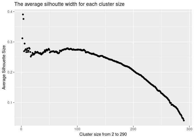
According to the graphic, three cluster seem to be the optimum with a value of 0.3906, although four and two clusters are also high with their average silhouette values of 0.3758 and 0.3118.
head(silhoutte_ergebnis$avg)

## [1] 0.3118969 0.3906218 0.3758216 0.2692193 0.2945250 0.2731856
To see which one is more appropriate, we plot the the cluster solutions from two to four and take a look at the corresponding silhouette values.
daten_bezirk$Cluster=silhouette(cutree(clust,3),distanz)[,1]
daten_bezirk$Neighbour=silhouette(cutree(clust,3),distanz)[,2]
daten_bezirk$Silhouette=silhouette(cutree(clust,3),distanz)[,3]
p1=ggplot(daten_bezirk)+geom_sf(aes(fill=factor(Cluster)))+labs(fill="Cluster")+ggtitle("Cluster assignment for 3 clusters")
p2=ggplot(daten_bezirk)+geom_sf(aes(fill=Silhouette))+ggtitle("Silhouette values for the regions")
grid.arrange(p1,p2,nrow=1)
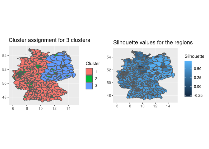
The three cluster solution divides germany into east germany, west germany and into big cities all over germany. In the right graphic the individual silhouette values for each constituencies are plotted. Values close to 1 indicate an optimal cluster assignment for this observation. In general cities and constituencies in the west have more negative values while the constituencies in the east have higher values.
sil1=silhouette(cutree(clust,3),distanz)
fviz_silhouette(sil1,print.summary=F)
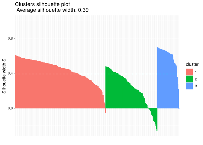 In addition we can plot the individual silhoutte values for each
constituencies. The dashed line is the average silhouette value over all
clusters. The constitutencies in east germany have high silhouette value
and seem to be well matched. The more problematic observations are in
cluster 2, which are the cities. A number of cities have negative
values, which indicate a bad cluster assignment. We therefore take a
look at the cluster solution for four groups.
In addition we can plot the individual silhoutte values for each
constituencies. The dashed line is the average silhouette value over all
clusters. The constitutencies in east germany have high silhouette value
and seem to be well matched. The more problematic observations are in
cluster 2, which are the cities. A number of cities have negative
values, which indicate a bad cluster assignment. We therefore take a
look at the cluster solution for four groups.
daten_bezirk$Cluster=silhouette(cutree(clust,4),distanz)[,1]
daten_bezirk$Neighbour=silhouette(cutree(clust,4),distanz)[,2]
daten_bezirk$Silhouette=silhouette(cutree(clust,4),distanz)[,3]
p1=ggplot(daten_bezirk)+geom_sf(aes(fill=factor(Cluster)))+labs(fill="Cluster")+ggtitle("Cluster assignment for 4 clusters")
p2=ggplot(daten_bezirk)+geom_sf(aes(fill=Silhouette))+ggtitle("Silhouette values for the regions")
grid.arrange(p1,p2,nrow=1)
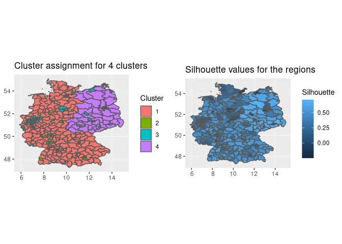 Once we increase the number of clusters by one, we see a split in the
city cluster. We have now a cluster for east geemany, west germany and
two city clusters. In city cluster two these cities tend to be located
in the south and west germany and are wealthier in general, as they
include cities like München, Frankfurt, Hamburg. City cluster three
includes cities in east germany and also cities in the west like
Hannover.
Once we increase the number of clusters by one, we see a split in the
city cluster. We have now a cluster for east geemany, west germany and
two city clusters. In city cluster two these cities tend to be located
in the south and west germany and are wealthier in general, as they
include cities like München, Frankfurt, Hamburg. City cluster three
includes cities in east germany and also cities in the west like
Hannover.
sil1=silhouette(cutree(clust,4),distanz)
fviz_silhouette(sil1,print.summary=F)
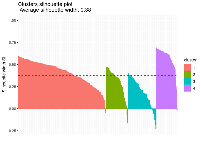 We here see negative silhouette values for the two city clusters 2 and
3.
We here see negative silhouette values for the two city clusters 2 and
3.
daten_bezirk$Cluster=silhouette(cutree(clust,2),distanz)[,1]
daten_bezirk$Neighbour=silhouette(cutree(clust,2),distanz)[,2]
daten_bezirk$Silhouette=silhouette(cutree(clust,2),distanz)[,3]
p1=ggplot(daten_bezirk)+geom_sf(aes(fill=factor(Cluster)))+labs(fill="Cluster")+ggtitle("Cluster assignment for 2 clusters")
p2=ggplot(daten_bezirk)+geom_sf(aes(fill=Silhouette))+ggtitle("Silhouette values for the regions")
grid.arrange(p1,p2,nrow=1)
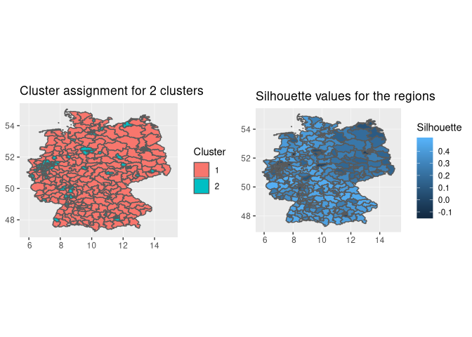 In the case for two clusters we have an urban cluster and a rural
cluster. Constituencies in east germany and cities in the south and west
have low silhouette values closer to zero or negative values.
In the case for two clusters we have an urban cluster and a rural
cluster. Constituencies in east germany and cities in the south and west
have low silhouette values closer to zero or negative values.
sil1=silhouette(cutree(clust,2),distanz)
#### braucht die Gruppenindikatoren und dann die Unähnlichkeitsmatrix
fviz_silhouette(sil1,print.summary=F)
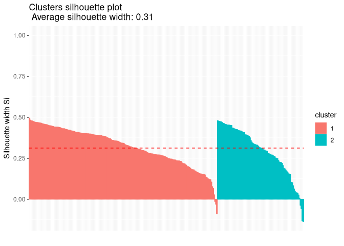
Comparing all those cluster solutions, the optimal number of clusters tend to be three or four. If we decide the optimal number just by the average silhouette width, three clusters solutions are optimal. In all those cluster solutions one could see the division into rural and urban constituencies and east and west germany. For the cluster solutoin with four groups, we can see an additional division for the urban constituencies. In addition some constituencies had negative silhouette values for all cluster solutions, which indicate in general a bad cluster assignment. This could be due to those observations being outliers in general, which would mean that they do not fit well into any real cluster solution. This would explain the fact, thtat some observations in the city cluster had negative silhouette values overall possible cluster solutions presented here. Other cluster like k-means could be used in addition to see how much the solutions are affected by the method used. k-means has the advantage to use an information based criteria like AIC for finding the optimal number of solutions.